The Geyokcha Array

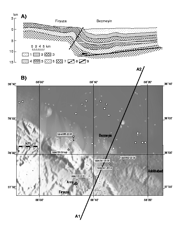
The Geyokcha array, located near the Iran-Turkmenistan border (Geyokcha regional map) , is an array of broadband & short-period seismographs deployed during 1993-94, as part of the IRIS-supported US-Soviet Joint Seismic Program. The array is located near the Kopet Dagh fault zone, marking the southern edge of the Eurasian Plate (Array detail) . There are a wide variety of local, regional, and teleseismic events recorded by the array, as well as a number of quarry and mining blasts. The array consists of nine three-component broadband stations and 36 short-period sensors  (Array detail) . For this exercise, we will be using only the broadband records. We will be using a segment of the array data from late 1993 through early 1994.
 
 

The Array Processing Software

We will be using a number of array-processing programs developed by Danny Harvey at University of Colorado, who is now present of BRTT, the company that sells and maintains Antelope. The processes are conveniently controlled through a GUI interface, called process_array , that is a tcl/tk script written originally Danny and modified some by G. Pavlis. From this script, we can run dbpick, to examine the orginal seismic data, dbap, to run the array processor, fk_script, to compute and display azimuth-slowness plots, st_script, to compute and display slowness-time plots, bm_script, to compute and display the array beams, and wr_script, to write the beams to disk. The GUI interface is a convenient way to control these subprocesses, and to display the array processing information on the screen.

To set yourself up to begin this exercise do the following:

1. Create a working directory to contain the data files for this exercise and cd to that directory.  Be warned this file is fairly large (30+ Mbytes when uncompressed) so be sure you have space available to hold the data.
2. Download the file.  Just  click here  to do this through your browser.
3. Assuming the current directory is the one you downloaded this file into, you need to uncompress the file with: gunzip array_exercise.tar.gz
4. Run tar to extract all the files contained in the tarball holding all the stuff you need:   tar xvf array_exercise.tar
5. You should now have a working database with everything in order.  Just type:  process_array
6. The following control panel should appear:

Note that the display shows the data being used for this exercise (gey) and the central reference station of the array (ORGH). The central portion of the interface shows a number of filter settings that we can use for calculating the array beams. The bottom of the display includes the buttons that control the sub-processes listed above.

(3) Start dbpick and dbap using the GUI interface buttons.

A dbpick window will open up, as well as two small xterm windows controlling dbpick and dbap. You might have to work a little to arrange the windows in some workable format.

(4) From the dbpick window, select one 3-component station to examine waveforms

sc ORGH:*

(later, if you want to examine all of the broadband verticals, you can display them using the command

sc *:HHZ,

or the short-period verticals, using

sc *:EHZ.

(5) Enable time fit to maximize the dbpick window

tfit

(6) Pick inital P-wave and S-wave arrivals, using the dbpick commands "Pick Arrivals" (See Gary's dbpick notes). Use filters as necessary to help identify phases--higher frequency for local events; lower frequencies for regional events and teleseisms.

(7) Run the azimuth-slowness script using the FK button on the process_array interface. A dbap display will open up, with "radar-screen" diagrams showing coherence as a function of azimuth and slowness. [Note: circles are at increments of 0.1 sec/km in slowness, and therefore non-linear in velocity]. Look for focused directions of energy arrival, reasonable apparent velocities, and agreement between P and S arrival directions. Repeat picks and/or filters as necessary to get coherent arrivals.

(8) Run the slowness-time script using the ST button on the process_array interface. Three plots showing slowness as a function of time in the vertical, radial, and transverse directions will appear, with a display of the reference station data (filtered) and beam data (filtered) for the best-fit arrival direction. Look for coherent arrivals around the P and S times. Repick arrivals and repeat (6) - (8) as necessary.

(9) Examine the beams using the BEAM button on the process_array interface. The display will show 12 traces (4 each for vertical, radial, and transverse). In each group, the top one shows filtered data for the reference station, filtered data for the beam, unfiltered data for the reference station, and unfiltered beam data.

(10) If you wish to save the beam data, use the WRITE button on the process_array interface. Caution: You may only do this ONCE for each event. If you try to write over pre-existing beam traces, the program will crash! Do not write unless you're sure that you've got your final beam traces!

(11) If you wish to make hard copies, you must edit the script fk_script, located in your g515 directory. Find the line

set psfile none

and change the "none" to a file name (e.g., plot.ps). The next time you run FK or ST, the program will write a parallel copy to disk as a postscript file, which can be printed directly. The file will be wiped out the next time you run the script. To run more efficiently, return the filename to "none" when you are done printing. If you have trouble getting a clear output on the color printer, you may want to try the unix command

setenv GRX_GAMMA 2.0

to get a better color map to the printer.

(12) To seek associations with earthquake tables, use the commands

oe /p/data/db/pde/pde_1993 or pde_1994

to open the event data base, and

ae

to seek an event associated with your picks. Note that at least one pick must be made before running this command.
 
 

Your Assignment

Process all the events you find in this database.   Use the array azimuth estimates and S-P times to get location estimates of each event.  We'll have a more precise catalog estimate at that time to compare what a computer program got to your rough solution.  Some additional things to focus on are:

1. The events in this set  span a range of distances from very close (I get ~ 5 km) to near teleseismic distances.  What differences do you see in the kinds of waveforms you see at different distances?
2. Try to use the array to help identify Pn, Pg, Sn, and Lg when this is appropriate.
3. On the regional events, once you have picks of some of the regional phases investigate the frequency dependence of the different phases and their "character" and report on this to the rest of the group.